
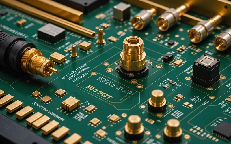
An RF PA evaluation kit is not a demo board. It is a calibration artifact. The measurements you take from it are only as valid as the calibration plane you establish and the accuracy of the de-embedding you apply between that plane and the device's RF ports. Hardware teams that plug in power, connect cables, and read numbers from a spectrum analyzer get data. Whether that data describes the PA or the evaluation board plus a combination of cable, connector, and PCB transmission line losses is a question that the setup methodology determines.
This guide covers evaluation kit setup, calibration approach, and the four measurement types that provide the most diagnostic value when deciding whether a PA meets system requirements. The focus is on Ka-band and Ku-band PA evaluation, where parasitic effects are large enough to make setup quality visible in the data.
Before Connecting Anything: Establish Your Calibration Reference Plane
The first decision in any PA evaluation is defining the calibration reference plane: the physical location in the signal chain where your measurement equipment is calibrated and where the stated measurement values apply. In a gain measurement, the reference plane is typically the PA's RF input and output ports at the evaluation board SMA or 2.92 mm connector interfaces.
A vector network analyzer calibrated at the test port end of your cables does not measure the PA. It measures the PA plus two connector interfaces, two cable assemblies from the calibration plane to the board connectors, and two PCB transmission line segments from the board connectors to the PA package. At 28 to 40 GHz, a 100 mm cable can introduce 0.3 to 0.8 dB of loss, and a SMA-to-2.92 mm connector transition adds reflection and loss that varies with connector quality and torque. These are not small errors. They systematically bias your gain and output power readings.
The correct procedure is to perform a SOLT (Short-Open-Load-Thru) or ECal calibration at the evaluation board's SMA or 2.92 mm connector interfaces, not at the VNA port. This requires a calibration kit specified for the connector type and frequency range, and the discipline to re-calibrate whenever cables are disturbed. For power measurements with a spectrum analyzer or power meter, establish the cable and connector loss at the frequencies of interest using the VNA before connecting the PA, and apply those loss values as corrections to every measurement.
A practical note: evaluation kits frequently include SMA connectors rated to 18 GHz on a board designed for Ka-band operation. The SMA connector is the bandwidth limit of the test setup, not the device. Replacing SMA connectors with 2.92 mm (K-type) connectors rated to 40 GHz and re-calibrating is a setup improvement that regularly recovers 0.5 to 1.5 dB of apparent gain at the top of the Ka-band.
Measurement 1: Small-Signal Gain and Input Return Loss vs. Frequency
The VNA S-parameter sweep gives you S21 gain and S11 input reflection across the full bandwidth of the evaluation board. Plot these versus frequency across the device's rated band and compare against the datasheet typical curves.
What to look for beyond the headline numbers: check gain flatness across the band. A specification for plus or minus 1.5 dB gain variation across 4 GHz of bandwidth is meaningfully different from a device that meets the spec on average but has a 3 dB gain dip at one specific frequency within the band. That dip may or may not fall within your intended channel bandwidth, but its presence indicates a resonance in the matching network or a substrate resonance in the package that has to be considered in a system where the channel occupies the full available bandwidth.
S11 input return loss tells you how well the PA input is matched to 50 ohms and therefore how much of your driver stage output power is actually entering the PA. A 10 dB return loss means 10% of power is reflected. At system level, reflected power from the PA input feeds backward through your driver, creating standing waves on the interconnect that cause gain variation with cable position. For a phased-array element where cable length variations are non-trivial, this matters for element-to-element gain consistency across the array.
Measurement 2: P1dB and Gain vs. Input Power Sweep
The output power versus input power sweep, commonly called a gain compression sweep, provides P1dB and the shape of the compression curve. Use a calibrated signal source, a well-characterized variable attenuator for step-by-step power control, and a power meter or spectrum analyzer with appropriate attenuation to avoid instrument compression.
Start the power sweep at least 20 dB below the expected P1dB input level and step in 1 dB increments. The early linear region establishes the small-signal gain reference. Compression begins visibly at roughly 3 to 5 dB below P1dB for most GaN devices. P1dB is the output power point at which the actual gain has fallen 1 dB below the small-signal extrapolation.
Pay attention to two non-obvious indicators. First, the shape of the compression curve above P1dB: a device that compresses sharply and then plateaus has different distortion characteristics than one that compresses gradually and continues to produce increasing output power with soft compression. Soft compression improves average efficiency at backoff under wideband modulation. Second, check whether the P1dB reading is stable under sustained drive. Applying CW drive at P1dB for 60 seconds and monitoring output power reveals whether the device exhibits thermal compression beyond the initial 1 dB: junction temperature rises during sustained drive and shifts the operating point. A device whose P1dB drops by more than 0.3 dB under 60 seconds of sustained CW drive is either running hot due to a thermal path problem on the evaluation board, or has insufficient backoff margin in the bias condition specified for the measurement.
Measurement 3: OIP3 Two-Tone Intermodulation
Two-tone OIP3 is the third-order output intercept point, the extrapolated power level at which the fundamental and third-order intermodulation products would have equal power. It describes the device's linearity headroom for multi-carrier and wideband modulated signal applications.
Set up two signal generators at frequencies f1 and f2 separated by a tone spacing relevant to your application, typically 1 to 100 MHz for satcom or 5G applications. Combine through a well-isolated power combiner. Both tones should enter the PA at identical power levels, backed off enough from P1dB that the third-order products are well above the spectrum analyzer noise floor but low enough that fifth-order products are negligible. A standard starting point is 10 dB below expected P1dB for each tone.
Measure the power difference between the fundamental and the closest third-order product (at 2f1-f2 and 2f2-f1). OIP3 equals output power per tone plus half the fundamental-to-IM3 ratio, in dB.
The practical insight OIP3 provides is headroom margin for the application's linearity requirement. A Ka-band PA intended for a high-throughput satellite link carrying 32-APSK or higher modulation needs OIP3 comfortably above the required output power, typically 8 to 12 dB of OIP3-to-P1dB ratio. An OIP3 that is only 5 dB above required output power will produce in-band distortion products that impair adjacent channel users in a multi-channel satellite transponder. OIP3 from a datasheet at a single operating point tells you very little without knowing the tone spacing, the operating temperature, and the supply voltage at which it was measured.
Measurement 4: AM-AM and AM-PM Curves
AM-PM, the phase rotation that accompanies gain compression, is the parameter most frequently omitted from PA evaluations and most consequential for 5G NR EVM compliance and phased-array calibration stability. Measuring it requires a VNA operating in a gain-phase measurement mode or a dedicated modulated signal testbed with a vector signal analyzer.
A simplified approach using a VNA: sweep input power at the center frequency of interest from small-signal to well past P1dB while recording the phase of S21 alongside the magnitude. The phase shift from small-signal to the compressed operating point is the AM-PM at that power level. Plot phase deviation versus output power. The slope of this curve in the region between 6 dB backoff and P1dB is the most operationally relevant segment for applications using OFDM waveforms.
Collect AM-PM data at minimum ambient temperature, nominal temperature, and elevated temperature if possible. Temperature-driven AM-PM variation is a reliability indicator for phased-array systems: if phase rotation shifts 3 degrees per 30-degree Celsius change in ambient, that variation must appear in the phased array's calibration overhead budget. A device that shows low AM-PM at room temperature but large AM-PM temperature sensitivity creates a calibration burden that the array control system must track continuously during thermal transients.
Bias Setup and Common Setup Errors
GaN HEMT evaluation requires correct quiescent bias before RF drive is applied. The gate bias is typically set to establish a specific quiescent drain current at a stated supply voltage. Deviating from the recommended quiescent point, even by 10 to 15%, shifts the device from the intended class of operation and alters gain, efficiency, and linearity characteristics.
Three setup errors account for most cases where evaluation data fails to reproduce datasheet values. First, cable loss not de-embedded: as described above, this biases gain and output power readings low. Second, quiescent bias set by input voltage rather than drain current: the threshold voltage of GaN devices varies by 100 to 200 mV between units, so setting a specific gate voltage without confirming the resulting drain current produces unit-to-unit setup inconsistency. Always set quiescent bias by confirming drain current, not gate voltage alone. Third, supply current limit set too conservatively: a power supply with a 2A current limit on a PA that draws 3A at peak RF output will clip the supply voltage during drive, causing gain and output power measurements that are incorrect because the device is supply-limited, not device-limited.
A well-executed evaluation on a properly calibrated bench, with these four measurements completed at the relevant operating temperature and bias conditions, provides the information needed to confidently compare a PA device against its datasheet and against the system link budget requirements. Shortcutting any one of the four measurements leaves a gap that often becomes visible only after the device has been designed into a board and the system-level performance review reveals the missing data.